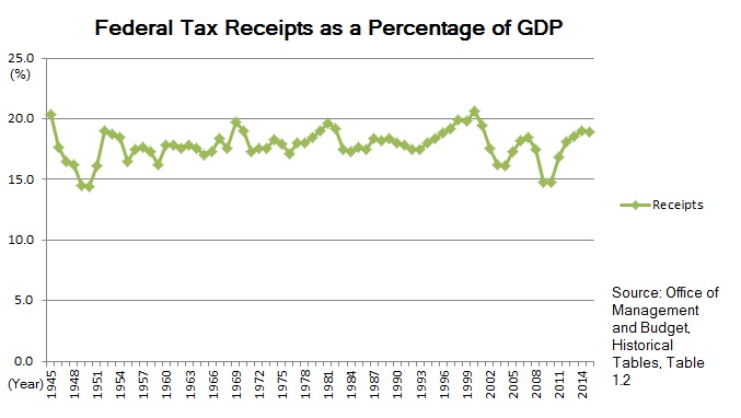
Hauser’s Curve           Image Credit: Wikimedia commons/Sugar-Baby-Love

With a Republican tax bill  having passed both houses of Congress and certain to be signed by the President, taxes and tax rates are the universal subject of the day. A critical empirical fact to consider in the debate is Hauser’s Law, as illustrated by Hauser’s curve above.

To Cut Or Not To Cut Taxes?

For some reason  progressives are stubbornly convinced that any cut in tax rates automatically equates to a cut in tax revenues. If you accept this claim, then as night follows day, any cut in tax rates will create larger federal deficits and a larger public debt in the absence of spending cuts. Isn’t this claim very obviously true?

Actually, the correct answer is an emphatic NO! The beginning of the neoliberal counterargument starts with Hauser’s Law. This is a purely empirical expression of a remarkable relationship between the U.S. GDP and federal tax revenues. The law states that no matter what the top marginal tax rates, federal tax receipts have stubbornly averaged 19.5% of GDP, plus or minus a few percent. In fact, the largest fluctuations from the 19.5% average are downward, and are associated as lagging indicators of recessions. By inspection of the plot above, you can see the largest downward fluctuations are lagging consequences of the recessions of 1945, 1949, 2001, and the Great Recession of 2007-2009. Clearly, if you want to maximize federal government revenues, you want to keep GDP growth as large as possible.

This remarkable lack of correlation between tax rates and federal tax receipts as a fraction of GDP is demonstrated in the plot below.

If a 90% plus top marginal tax rate as in the 1950s is not sufficient to increase the share of GDP taken by the government, what would be the point of increasing tax rates?

Why does this remarkable empirical law hold? As far as I know, no one has given a dispositive reason, although it is very easy to think of possible explanations. One highly likely exposition is the economically destructive nature of increased government allocation of scarce economic resources. One inevitable result of increasing tax rates is government gets to allocate a larger share of GDP to its own ends, and companies and private households allocate less. Not only do government bureaucrats tend to direct economic assets to where the economy does not really need them, but it denies those same resources to private companies and households. The entire purpose of companies in the pursuit of profits is to efficiently invest assets to meet the needs of the population, and to help manage the supply-demand balances on which the health of the economy depends.

This couples government waste with opportunity costs for the economy. As economic growth is reduced due to government interference with the economy, GDP growth together with increases in taxable income and income tax receipts declines. As a result, although tax rates may have increased, government revenue is reduced from what it otherwise would be because of the smaller taxable GDP.

The Link Between Economic Growth And Tax Revenue With Government Expenditures: The Rahn Curve

Since U.S. tax revenues  depend only on the size of the GDP and not on tax rates, the very next question should be just how does GDP change with increasing or decreasing tax rates? The answer comes from a theoretical construct called the Rahn curve, which is nevertheless partially verified by historical economic data. The theoretical notion of the Rahn curve is illustrated below.

The basic idea is that there is an optimal size of government in terms of the fraction of GDP it spends. If the spending is less than this optimum, then government does not support infrastructure and government’s defense of the social contract enough to allow increased economic growth. As government spending goes toward zero percent of GDP, usable roads and bridges begin to disappear and we enter Thomas Hobbes’ state of nature, a “war of all against all.” As social cooperation decreases, so does economic growth. Call this the growing branch of the Rahn curve, since GDP growth increases with government size on this branch of the Rahn curve. This is the branch progressives believe we almost always live on.

Now suppose government spending as a share of GDP is greater than the optimal level. Then as government pulls more assets away from the private economy, economic growth rates fall. The explanation for this is much the same as in my speculation above for the reasons why Hauser’s law works. Government officials are almost always lousy investors, primarily because their interests are different from profit-seeking companies. Companies are forced to create more wealth than they consume; otherwise they go out of existence via bankruptcy. Government officials, both elected and appointed, on the other hand usually are not nearly as concerned with the economic effects as with the political ones. An excellent recent example of this was the federal investments in the solar power firm Solyndra, in which the government lost at least $535 million. As a result, as the share of GDP represented by government spending increases, capital is increasingly misallocated and GDP growth falls. Call this the declining branch of the Rahn curve. It is the branch on which neoliberals believe we have been living for many decades.

So what is the actual reality? Do we have any data that can tell us what the truth is? In fact, we can construct a scatter plot of each fiscal quarter’s annual percent change of the real GDP versus that quarter’s annualized government expenditures as a percent of GDP. The data is taken from the Federal Reserve Economic Database, using data from every quarter from the second quarter of 1959 to the third quarter of 2017. The clustering of the data points should define a portion of the Rahn curve. The result is shown below.

Clearly, the slope of any trend line to this scatter plot would be negative, demonstrating that at least since the second quarter of 1959 we have been on the declining branch of the Rahn curve. Also clear is that whatever the optimum size of government spending, it is somewhat less than 19% of GDP. It is also obvious that while government revenue had been limited to around 19.5% of GDP, almost all quarters during this period had government expenditures far in excess of that amount. Hence our humongous national debt that is around 105% of GDP.

What the data is shouting at us is that we are living in the neoliberal universe, not the progressive alternative universe. Should we increase tax rates, politicians (being what they are) will almost certainly increase spending, from which Rahn’s curve predicts we would have smaller — perhaps even negative — growth rates. Rahn’s curve is coupled to Hauser’s curve because of the modern relationship between government revenues and expenditures. American politicians can not resist spending all available revenues and a lot more. Rahn’s curve then tells us that as expenditures increase, the GDP growth rate decreases. Hauser’s law in turn tells us as the growth in the GDP decreases, the increase in government revenues decreases in tandem. If the politicians’ increases in spending are enough to create perpetual deficit spending, eventually the decreases in GDP growth will make the growth rate negative, and actually decrease government revenues. The descent into the financial abyss would then be very rapid.

President Obama’s administration left us very close to that dreadful destiny. A plot I have shown over and over again demonstrates how our long-term secular growth rate has almost reached zero. [The word “secular” is used here to mean averaged over the business cycle.] It was produced by a Gallup Organization economist, Jonathon Rothwell, in a report that you can download in PDF format here. What he did was to calculate a moving time average of real per capita GDP over ten year periods. Doing this, Rothwell was able to average over the business cycle to show long term trends. Plotting that moving time average produced the plot below.

Clearly, the dashed linear trend line since 1966 has negative slope, with the actual 10-year average in 2016 getting fearfully close to zero. One can argue that over the Reagan and Clinton regimes the decay plateaued, but the trend outside those two administrations is definitely downwards. Once the per capita GDP growth rate actually hits zero, Hauser’s law tells us government revenues will also start to decline, no matter what the tax rates. At that point the federal budget deficit and the public debt will begin to explode, with unpredictable results for the survival of the United States.

The Republican tax reform bill is one attempt to stave off this disaster by rekindling economic growth, thereby producing increased government revenues. President Trump has also been effective in increasing the growth rate by his partial demolition of the regulatory state through executive orders. By dint of reducing the regulatory burdens on companies, he has been able to rekindle their optimism that increased growth is indeed possible, and to motivate them to increase investment and production. As a result, according to the Federal Reserve, the real GDP growth rate increased to 3.1% in the second quarter of this year and to 3.3% in the third quarter. This follows the poor economic performance of President Obama, who was the first American president since Herbert Hoover who did not have a single year during his regime with at least 3% annual growth or better.

Will Tax Reforms And Cuts Be Enough To Reduce Federal Budget Deficits?

Alas,  it is highly unlikely that tax reforms will all by themselves halt the growth of federal deficits. The problem is illustrated by another graph I use a lot, shown below.

The red crosses are historical data points of federal expenditures on mandatory entitlements plus interest on the national debt. The blue curve is a nonlinear least-squares fit of an exponential function to the data. The purple boxes are the data points for total federal revenues, and the green curve is an exponential fit to that data. I then extrapolated the fitted functions to the year 2045 to see what would happen if nothing changes. What the plot tells us is that by April 2031, just the expenditures on mandatory entitlements plus interest on the national debt alone would be enough to absorb every single penny of government revenues. There would be nothing left over to defend the country, to fund the federal court system, to fund the Congress, or to do anything else!

What tax reform and cuts would do is to increase the growth rate of the green revenue curve, pushing it up, and to postpone the date when expenditures would catch up to bankrupt the U.S. government. However, the exponential growth rate of expenditures is so much greater than that of revenues, tax reform would have to generate a huge increase in GDP growth to generate a large enough revenue growth rate to solve the problem. Tax reforms and cuts can greatly improve the economy to ameliorate the problem and delay disaster. However, the rate of growth of government spending, specifically that for mandatory entitlements (Medicare, Medicaid, and Social Security), is much too large for us to ignore. The creation of additional mandatory entitlements, e.g. Obamacare or a federally guaranteed national income advocated by many progressives, would only make catastrophe all the more certain.

Views: 5,017

GO TO HOME

Sharing is caring!